Mapping data across geographies • hpa.spatial

library(hpa.spatial)
library(dplyr)
library(tidyr)
library(stringr)
library(ggplot2)

“Mapping” in the title is talking about more of a purr::map() than a mapview::mapview() kind of “map”. The objective is to appropriately move data from one set of polygons to another. It is heavily inspired by the Australian context and uses population-based correspondence tables between geographies to perform this “mapping”.

The problem

A task that often comes up when working with spatial data is to move data across geographies for presentation. Aggregating up from SA2s to SA3s can be straight forward, but mapping data between partially (but not completely) overlapping geographies can be trickier. For example, not all SA2s are wholly contained within a single local hospital network (LHN). In these cases, it we may want to take a couple different approaches to moving the data from SA2 to LHN and presenting that data. This also happens between editions of the ASGS, say from the 2011 to the 2016 edition for SA2s.

The solutions

Solution 1: Map data from one geography to another based on population

The Australian Bureau of Statistics (ABS) release correspondence tables which allow the user to estimate the proportion of cross over between a pair of geographies (based on residential population).

These are helpful when mapping between geographies which they release editions for. For example, between the 2011 and 2016 edition of SA2s.

sa2_cg <- get_correspondence_tbl(
  from_area = "sa2",
  from_year = 2011,
  to_area = "sa2",
  to_year = 2016
)

sa2_cg
#> # A tibble: 2,426 × 3
#>    SA2_MAINCODE_2011 SA2_MAINCODE_2016 ratio
#>    <chr>             <chr>             <dbl>
#>  1 101011001         101051539             1
#>  2 101011002         101051540             1
#>  3 101011003         101061541             1
#>  4 101011004         101061542             1
#>  5 101011005         101061543             1
#>  6 101011006         101061544             1
#>  7 101021007         101021007             1
#>  8 101021008         101021008             1
#>  9 101021009         101021009             1
#> 10 101021010         101021010             1
#> # ℹ 2,416 more rows

Some of the SA2 codes from 2011 will be split into more than one SA2 code in the 2016 edition.

sa2_cg |> filter(ratio != 1)
#> # A tibble: 461 × 3
#>    SA2_MAINCODE_2011 SA2_MAINCODE_2016   ratio
#>    <chr>             <chr>               <dbl>
#>  1 102021047         102021047         0.993  
#>  2 102021047         102021055         0.00658
#>  3 104011082         104011082         1.00   
#>  4 107011130         107011545         0.482  
#>  5 107011130         107011546         0.362  
#>  6 107011130         107011547         0.157  
#>  7 107041144         107041144         1.00   
#>  8 107041149         107041548         0.449  
#>  9 107041149         107041549         0.551  
#> 10 109011172         109011172         1.00   
#> # ℹ 451 more rows

The map_data_with_correspondence() uses these correspondence tables to map values from one geography to another. It can be used to map rows of data (using the ratio as a probability of assignment to the new area). For example, if we pass two values from this code to map_data_with_correspondence() and ask it to map to the 2016 edition, these (may) be distributed across to different geographies. This considers each code-value pair as a single unit to be allocated to a new geography and is specified by the value_type argument.

map_data_with_correspondence(
  codes = c(107011130, 107011130),
  values = c(1, 4),
  from_area = "sa2",
  from_year = 2011,
  to_area = "sa2",
  to_year = 2016,
  value_type = "units",
  seed = 2
)
#> # A tibble: 2 × 2
#>   SA2_MAINCODE_2016 values
#>   <chr>              <dbl>
#> 1 107011545              1
#> 2 107011546              4

However, if the code-value pairs are aggregate values (i.e. number of car crashes in that SA2), then it would be preferable to split them and then aggregate up again in the new geographies. This is what happens when we pass “aggregate” values with value_type = "aggs"

map_data_with_correspondence(
  codes = 107011130,
  values = 10,
  from_area = "sa2",
  from_year = 2011,
  to_area = "sa2",
  to_year = 2016,
  value_type = "aggs"
)
#> # A tibble: 3 × 2
#>   SA2_MAINCODE_2016 values
#>   <chr>              <dbl>
#> 1 107011545           4.82
#> 2 107011546           3.62
#> 3 107011547           1.57

Solution 2: Adjust your geography so suit.

In some cases, you may be given data on the SA2 level but want to visualise on the LHN level. SA2s are almost always completely contained within an LHN but this isn’t always the case. If it’s still important to be able to see differences between SA2s but also differences between LHNs, it might be best to split those particular SA2s where they cross LHN boundaries.

custom_geo <- create_child_geo(
  child_geo = get_polygon("sa22011"),
  parent_geo = get_polygon("LHN")
)
#> The data for the Local Hospital Networks (LHN) are from here: <https://hub.arcgis.com/datasets/ACSQHC::local-hospital-networks/explore>

custom_geo |>
  filter(stringr::str_detect(sa2_code_2011, "210041241")) |>
  ggplot() +
  geom_sf(alpha = 1, aes(fill = sa2_code_2011), size = 10, col = "transparent") +
  geom_sf(
    data = filter(get_polygon("LHN"), LHN_Name %in% c("Brimbank Melton", "Hume Moreland")),
    aes(fill = LHN_Name),
    col = "black",
    linetype = "dashed",
    size = 10,
    alpha = 0.4
  ) +
  labs(fill = "") +
  theme_bw()
#> The data for the Local Hospital Networks (LHN) are from here: <https://hub.arcgis.com/datasets/ACSQHC::local-hospital-networks/explore>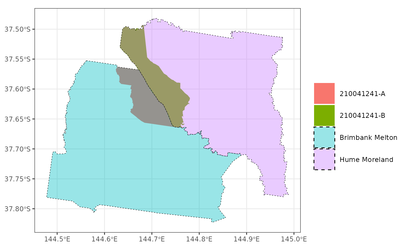

In this graphic, the original SA2 (210041241) that crosses the LHN boundary (Brimbank Melton and Hume Moreland) is split into two parts (A and B) at the boarder.

We can map data to this new geography and so that we can visualise differences between SA2s while maintaining a separation between LHNs.

Mapping grouped data

Sometimes, we may have data for groups, with values for each group within each geography and want to map these to a new geography. map_data_with_correspondence() can handle these groups nicely with the groups argument. Also in this example, we show off that you can pass the input data as .data and reference its columns for the codes and values arguments rather than passing them as vectors.

sa2_2011_data <-
  get_polygon("sa22011") |>
  as_tibble() |>
  select(sa2_code_2011) |>
  mutate(
    ages_00_to_11 = rnorm(n = max(n()), mean = 10, sd = 2),
    ages_12_to_24 = rnorm(n = max(n()), mean = 20, sd = 4),
    ages_25_to_64 = rnorm(n = max(n()), mean = 25, sd = 5),
    ages_65_plus = rnorm(n = max(n()), mean = 40, sd = 8)
  ) |>
  pivot_longer(
    !sa2_code_2011,
    names_to = "agegrp",
    values_to = "outcome_var",
    names_transform = ~ str_remove(.x, "ages_") |>
      str_replace("_to_", "-") |>
      str_replace("_plus", "+")
  )
#> Reading sa22011 file found in /tmp/RtmpmPTdTU

sa2_2016_data <- map_data_with_correspondence(
  .data = sa2_2011_data,
  codes = sa2_code_2011,
  values = outcome_var,
  groups = agegrp,
  from_area = "sa2",
  from_year = 2011,
  to_area = "sa2",
  to_year = 2016,
  value_type = "aggs"
)

sa2_2016_data
#> # A tibble: 9,212 × 3
#>    SA2_MAINCODE_2016 outcome_var agegrp
#>    <chr>                   <dbl> <chr> 
#>  1 101021007                6.36 00-11 
#>  2 101021008                9.51 00-11 
#>  3 101021009                9.51 00-11 
#>  4 101021010                9.43 00-11 
#>  5 101021011                8.89 00-11 
#>  6 101021012               11.3  00-11 
#>  7 101031013               14.1  00-11 
#>  8 101031014                6.74 00-11 
#>  9 101031015               11.0  00-11 
#> 10 101031016                6.27 00-11 
#> # ℹ 9,202 more rows